Skip to content

2D Model

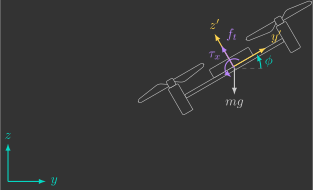
We begin by deriving the differential equations that describe the 2D dynamics of a quadcopter. Starting with a simplified two-dimensional model reduces the mathematical complexity and provides a more intuitive understanding of the system. This model serves as an essential first step for visualizing how the inputs affect the outputs.


Introduction

The 2D model has three degrees of freedom (two translational and one rotational). Therefore, we must derive six differential equations (two for each degree of freedom)(1).

  1. For clarity, we will use the following colors and notation:
    • \({\color{var(--c1)} x}\) — States (inertial frame)
    • \({\color{var(--c3)} x\,'}\) — States (body-fixed frame)
    • \({\color{var(--c2)} u}\) — Inputs
    • \(m\) — Constants

We will derive this model from four different perspectives, in the following order:

Order Notation Positions Velocities
1 Scalar \( y \quad z \quad \phi \) \( v_y \quad v_z \quad \omega_x \)
2 \( y \quad z \quad \phi \) \( v^{'}_y \quad v^{'}_z \quad \omega^{'}_x \)
3 Vector \( y \quad z \quad \phi \) \( v_y \quad v_z \quad \omega_x \)
4 \( y \quad z \quad \phi \) \( v^{'}_y \quad v^{'}_z \quad \omega^{'}_x \)

Although the formulations become progressively more complex, when we extend the model to 3D, the fourth (and final) perspective ultimately becomes the simplest one.


Scalar notation

Newton's second law for translation and rotation, written in scalar form, is:

\[ \left\{ \begin{array}{l} \sum f = m a \\ \sum \tau = I \alpha \end{array} \right. \]

These equations must be applied independently to each degree of freedom.

Inertial frame

We begin by expressing both the positions and the velocities in the inertial frame. The system states are therefore \({\color{var(--c1)}y}\), \({\color{var(--c1)}z}\), \({\color{var(--c1)}\phi}\), \({\color{var(--c1)}v_y}\), \({\color{var(--c1)}v_z}\), and \({\color{var(--c1)}\omega_x}\).

Exercise 8.1

Derive the kinematic equations, that is, the time derivatives of the positions (\({\color{var(--c1)}y}\), \({\color{var(--c1)}z}\), and \({\color{var(--c1)}\phi}\)) as functions of the system states.

a) Express \({\color{var(--c1)}\dot{y}}\) in terms of the system states.
\[ {\color{var(--c1)}\dot{y}} = {\color{var(--c1)}v_y} \]
b) Express \({\color{var(--c1)}\dot{z}}\) in terms of the system states.
\[ {\color{var(--c1)}\dot{z}} = {\color{var(--c1)}v_z} \]
c) Express \({\color{var(--c1)}\dot{\phi}}\) in terms of the system states.
\[ {\color{var(--c1)}\dot{\phi}} = {\color{var(--c1)}\omega_x} \]

Exercise 8.2

Derive the kinetic equations, that is, the time derivatives of the velocities (\({\color{var(--c1)}v_y}\), \({\color{var(--c1)}v_z}\), and \({\color{var(--c1)}\omega_x}\)) as functions of the system states.

Hint: Apply Newton's second law independently to each degree of freedom in the inertial frame.

a) Express \({\color{var(--c1)}\dot{v}_y}\) in terms of the system states.
\[ \begin{align*} \sum {\color{var(--c1)}f_y} &= m {\color{var(--c1)}a_y} \\ -{\color{var(--c2)}f_t}\sin{\color{var(--c1)}\phi} &= m{\color{var(--c1)}\dot{v}_y} \\ {\color{var(--c1)}\dot{v}_y} &= -\frac{1}{m}\sin{\color{var(--c1)}\phi}\,{\color{var(--c2)}f_t} \end{align*} \]
b) Express \({\color{var(--c1)}\dot{v}_z}\) in terms of the system states.
\[ \begin{align*} \sum {\color{var(--c1)}f_z} &= m {\color{var(--c1)}a_z} \\ {\color{var(--c2)}f_t}\cos{\color{var(--c1)}\phi} - mg &= m{\color{var(--c1)}\dot{v}_z} \\ {\color{var(--c1)}\dot{v}_z} &= -g + \frac{1}{m}\cos{\color{var(--c1)}\phi}\,{\color{var(--c2)}f_t} \end{align*} \]
c) Express \({\color{var(--c1)}\dot{\omega}_x}\) in terms of the system states.
\[ \begin{align*} \sum {\color{var(--c1)}\tau_x} &= I_{xx}{\color{var(--c1)}\alpha_x} \\ {\color{var(--c2)}\tau_x} &= I_{xx}{\color{var(--c1)}\dot{\omega}_x} \\ {\color{var(--c1)}\dot{\omega}_x} &= \frac{1}{I_{xx}}{\color{var(--c2)}\tau_x} \end{align*} \]

By combining the kinematic and kinetic equations, we obtain the complete system dynamics:

\[ \left\{ \begin{array}{l} {\color{var(--c1)}\dot{y}} = {\color{var(--c1)}v_y} \\ {\color{var(--c1)}\dot{z}} = {\color{var(--c1)}v_z} \\ {\color{var(--c1)}\dot{\phi}} = {\color{var(--c1)}\omega_x} \\ {\color{var(--c1)}\dot{v}_y} = -\dfrac{1}{m}\sin{\color{var(--c1)}\phi}\,{\color{var(--c2)}f_t} \\ {\color{var(--c1)}\dot{v}_z} = -g + \dfrac{1}{m}\cos{\color{var(--c1)}\phi}\,{\color{var(--c2)}f_t} \\ {\color{var(--c1)}\dot{\omega}_x} = \dfrac{1}{I_{xx}}{\color{var(--c2)}\tau_x} \end{array} \right. \]

Body-fixed frame

Another way to formulate the problem is to express the positions in the inertial frame while expressing the velocities in the body-fixed frame. The system states then become \({\color{var(--c1)}y}\), \({\color{var(--c1)}z}\), \({\color{var(--c1)}\phi}\), \({\color{var(--c3)}v_y\,'}\), \({\color{var(--c3)}v_z\,'}\), and \({\color{var(--c3)}\omega_x\,'}\).

This formulation is commonly used because it is more natural to describe velocities in the frame fixed to the drone. Moreover, most onboard sensors (accelerometers, gyroscopes, proximity sensors, optical flow sensors, etc.) are rigidly attached to the vehicle and aligned with this frame. As we will see, however, the resulting equations become slightly more complex and less intuitive.

Exercise 8.3

Derive the kinematic equations, that is, the time derivatives of the positions (\({\color{var(--c1)}y}\), \({\color{var(--c1)}z}\), and \({\color{var(--c1)}\phi}\)) in terms of the system states.

Hint: Recall the rotation matrices introduced before and note that the \({\color{var(--c1)}x}\) and \({\color{var(--c3)}x\,'}\) axes are aligned.

a) Express \({\color{var(--c1)}\dot{y}}\) in terms of the system states.
\[ \begin{bmatrix} {\color{var(--c3)}v_y\,'} \\ {\color{var(--c3)}v_z\,'} \end{bmatrix} = \underbrace{ \begin{bmatrix} \cos{\color{var(--c1)}\phi} & \sin{\color{var(--c1)}\phi} \\ -\sin{\color{var(--c1)}\phi} & \cos{\color{var(--c1)}\phi} \end{bmatrix} }_{R} \begin{bmatrix} {\color{var(--c1)}\dot{y}} \\ {\color{var(--c1)}\dot{z}} \end{bmatrix} \qquad \longrightarrow \qquad \begin{bmatrix} {\color{var(--c1)}\dot{y}} \\ {\color{var(--c1)}\dot{z}} \end{bmatrix} = \underbrace{ \begin{bmatrix} \cos{\color{var(--c1)}\phi} & -\sin{\color{var(--c1)}\phi} \\ \sin{\color{var(--c1)}\phi} & \cos{\color{var(--c1)}\phi} \end{bmatrix} }_{R^{-1}} \begin{bmatrix} {\color{var(--c3)}v_y\,'} \\ {\color{var(--c3)}v_z\,'} \end{bmatrix} \]
\[ {\color{var(--c1)}\dot{y}} = {\color{var(--c3)}v_y\,'}\cos{\color{var(--c1)}\phi} - {\color{var(--c3)}v_z\,'}\sin{\color{var(--c1)}\phi} \]
b) Express \({\color{var(--c1)}\dot{z}}\) in terms of the system states.
\[ \begin{bmatrix} {\color{var(--c3)}v_y\,'} \\ {\color{var(--c3)}v_z\,'} \end{bmatrix} = \underbrace{ \begin{bmatrix} \cos{\color{var(--c1)}\phi} & \sin{\color{var(--c1)}\phi} \\ -\sin{\color{var(--c1)}\phi} & \cos{\color{var(--c1)}\phi} \end{bmatrix} }_{R} \begin{bmatrix} {\color{var(--c1)}\dot{y}} \\ {\color{var(--c1)}\dot{z}} \end{bmatrix} \qquad \longrightarrow \qquad \begin{bmatrix} {\color{var(--c1)}\dot{y}} \\ {\color{var(--c1)}\dot{z}} \end{bmatrix} = \underbrace{ \begin{bmatrix} \cos{\color{var(--c1)}\phi} & -\sin{\color{var(--c1)}\phi} \\ \sin{\color{var(--c1)}\phi} & \cos{\color{var(--c1)}\phi} \end{bmatrix} }_{R^{-1}} \begin{bmatrix} {\color{var(--c3)}v_y\,'} \\ {\color{var(--c3)}v_z\,'} \end{bmatrix} \]
\[ {\color{var(--c1)}\dot{z}} = {\color{var(--c3)}v_y\,'}\sin{\color{var(--c1)}\phi} + {\color{var(--c3)}v_z\,'}\cos{\color{var(--c1)}\phi} \]
c) Express \({\color{var(--c1)}\dot{\phi}}\) in terms of the system states.
\[ {\color{var(--c1)}\dot{\phi}} = {\color{var(--c3)}\omega_x\,'} \]

Exercise 8.4

Derive the kinetic equations, that is, the time derivatives of the velocities (\({\color{var(--c3)}v_y\,'}\), \({\color{var(--c3)}v_z\,'}\), and \({\color{var(--c3)}\omega_x\,'}\)) in terms of the system states.

Hint: Apply Newton's second law independently to each degree of freedom in the body-fixed frame.

a) Express \({\color{var(--c3)}\dot{v}_y\,'}\) in terms of the system states.
\[ \begin{align*} \sum {\color{var(--c3)}f_y\,'} &= m{\color{var(--c3)}a_y\,'} \\ -mg\sin{\color{var(--c1)}\phi} &= m\left({\color{var(--c3)}\dot{v}_y\,'} - {\color{var(--c3)}v_z\,'\omega_x\,'}\right) \\ {\color{var(--c3)}\dot{v}_y\,'} &= {\color{var(--c3)}v_z\,'\omega_x\,'} - g\sin{\color{var(--c1)}\phi} \end{align*} \]
b) Express \({\color{var(--c3)}\dot{v}_z\,'}\) in terms of the system states.
\[ \begin{align*} \sum {\color{var(--c3)}f_z\,'} &= m{\color{var(--c3)}a_z\,'} \\ {\color{var(--c2)}f_t} - mg\cos{\color{var(--c1)}\phi} &= m\left({\color{var(--c3)}\dot{v}_z\,'} + {\color{var(--c3)}v_y\,'\omega_x\,'}\right) \\ {\color{var(--c3)}\dot{v}_z\,'} &= -{\color{var(--c3)}v_y\,'\omega_x\,'} - g\cos{\color{var(--c1)}\phi} + \frac{1}{m}{\color{var(--c2)}f_t} \end{align*} \]
c) Express \({\color{var(--c3)}\dot{\omega}_x\,'}\) in terms of the system states.
\[ \begin{align*} \sum {\color{var(--c3)}\tau_x\,'} &= I_{xx}{\color{var(--c3)}\alpha_x\,'} \\ {\color{var(--c2)}\tau_x} &= I_{xx}{\color{var(--c3)}\dot{\omega}_x\,'} \\ {\color{var(--c3)}\dot{\omega}_x\,'} &= \frac{1}{I_{xx}}{\color{var(--c2)}\tau_x} \end{align*} \]

By combining the kinematic and kinetic equations, we obtain the complete system dynamics:

\[ \left\{ \begin{array}{l} {\color{var(--c1)}\dot{y}} = {\color{var(--c3)}v_y\,'}\cos{\color{var(--c1)}\phi} - {\color{var(--c3)}v_z\,'}\sin{\color{var(--c1)}\phi} \\ {\color{var(--c1)}\dot{z}} = {\color{var(--c3)}v_y\,'}\sin{\color{var(--c1)}\phi} + {\color{var(--c3)}v_z\,'}\cos{\color{var(--c1)}\phi} \\ {\color{var(--c1)}\dot{\phi}} = {\color{var(--c3)}\omega_x\,'} \\ {\color{var(--c3)}\dot{v}_y\,'} = {\color{var(--c3)}v_z\,'\omega_x\,'} - g\sin{\color{var(--c1)}\phi} \\ {\color{var(--c3)}\dot{v}_z\,'} = - {\color{var(--c3)}v_y\,'\omega_x\,'} - g\cos{\color{var(--c1)}\phi} + \frac{1}{m}{\color{var(--c2)}f_t} \\ {\color{var(--c3)}\dot{\omega}_x\,'} = \frac{1}{I_{xx}}{\color{var(--c2)}\tau_x} \end{array} \right. \]

The terms \({\color{var(--c3)}v_z,'\omega_x,'}\) and \({\color{var(--c3)}v_y,'\omega_x,'}\) are pseudo-acceleration terms that appear because the equations are expressed in the drone's rotating (non-inertial) body-fixed frame.


Vector notation

Newton's second law for translation and rotation, written in vector form, is given by:

\[ \left\{ \begin{array}{l} \sum {\color{var(--c1)}\vec{f}} = \dfrac{d}{dt}{\color{var(--c1)}\vec{p}} \\[2mm] \sum {\color{var(--c1)}\vec{\tau}} = \dfrac{d}{dt}{\color{var(--c1)}\vec{h}} \end{array} \right. \]

Where \({\color{var(--c1)}\vec{p}}\) and \({\color{var(--c1)}\vec{h}}\) are the linear and angular momentum vectors, respectively:

\[ \left\{ \begin{array}{l} {\color{var(--c1)}\vec{p}} = m{\color{var(--c1)}\vec{v}} \\[2mm] {\color{var(--c1)}\vec{h}} = I{\color{var(--c1)}\vec{\omega}} \end{array} \right. \]

Although \(m\) remains a scalar representing the mass of the body, \(I\) is now the inertia matrix, which contains the moments of inertia about the three rotational axes:

\[ I = \begin{bmatrix} I_{xx} & 0 & 0 \\ 0 & I_{yy} & 0 \\ 0 & 0 & I_{zz} \end{bmatrix} \]

Since we are now working with vectors, these equations can be applied simultaneously to all degrees of freedom.

Inertial frame

We begin by defining the gravity vector \({\color{var(--c1)}\vec{g}}\) in the inertial frame and the drone's force and torque vectors, \({\color{var(--c3)}\vec{f}_d\,'}\) and \({\color{var(--c3)}\vec{\tau}_d\,'}\), in the body-fixed frame:

\[ {\color{var(--c1)}\vec{g}} = \begin{bmatrix} 0 \\ 0 \\ g \end{bmatrix} \qquad {\color{var(--c3)}\vec{f_d}\,'} = \begin{bmatrix} 0 \\ 0 \\ {\color{var(--c2)}f_t} \end{bmatrix} \qquad {\color{var(--c3)}\vec{\tau_d}\,'} = \begin{bmatrix} {\color{var(--c2)}\tau_x} \\ 0 \\ 0 \end{bmatrix} \]

This choice is convenient because each vector is naturally aligned with its corresponding frame, making it much easier to express.

Exercise 8.5

Exercise 8.6

Derive the vector kinetic equations, that is, the time derivatives of the velocity vectors (\({\color{var(--c1)}\vec{v}}\) and \({\color{var(--c1)}\vec{\omega}}\)) in terms of the net force and torque vectors.

a) Express \({\color{var(--c1)}\dot{\vec{v}}}\) in terms of \(\sum{\color{var(--c1)}\vec{f}}\).
\[ \begin{align*} \sum {\color{var(--c1)}\vec{f}} &= \frac{d}{dt}{\color{var(--c1)}\vec{p}} \\ \sum {\color{var(--c1)}\vec{f}} &= \frac{d}{dt}\left(m{\color{var(--c1)}\vec{v}}\right) \\ \sum {\color{var(--c1)}\vec{f}} &= m{\color{var(--c1)}\dot{\vec{v}}} \\ {\color{var(--c1)}\dot{\vec{v}}} &= \frac{1}{m}\sum{\color{var(--c1)}\vec{f}} \end{align*} \]
b) Express \({\color{var(--c1)}\dot{\vec{\omega}}}\) in terms of \(\sum{\color{var(--c1)}\vec{\tau}}\).
\[ \begin{align*} \sum {\color{var(--c1)}\vec{\tau}} &= \frac{d}{dt}{\color{var(--c1)}\vec{h}} \\ \sum {\color{var(--c1)}\vec{\tau}} &= \frac{d}{dt}\left(I{\color{var(--c1)}\vec{\omega}}\right) \\ \sum {\color{var(--c1)}\vec{\tau}} &= I{\color{var(--c1)}\dot{\vec{\omega}}} \\ {\color{var(--c1)}\dot{\vec{\omega}}} &= I^{-1}\sum{\color{var(--c1)}\vec{\tau}} \end{align*} \]

You should have obtained

\[ \left\{ \begin{array}{l} {\color{var(--c1)}\dot{\vec{v}}}=\dfrac{1}{m}\sum{\color{var(--c1)}\vec{f}} \\[2mm] {\color{var(--c1)}\dot{\vec{\omega}}}=I^{-1}\sum{\color{var(--c1)}\vec{\tau}} \end{array} \right. \]

These equations are completely general: they describe the translational and rotational motion of any rigid body. The only quantities that change from one system to another are the net force and net torque.

Exercise 8.7

Substitute the force and torque vectors defined at the beginning of this section to derive the kinetic equations.

Hint: Be careful with the reference frame in which each vector is expressed.

a) Express \({\color{var(--c1)}\dot{\vec{v}}}\) in terms of the system states.
\[ \begin{align*} {\color{var(--c1)}\dot{\vec{v}}} &= \frac{1}{m}\sum{\color{var(--c1)}\vec{f}} \\ {\color{var(--c1)}\dot{\vec{v}}} &= \frac{1}{m}\left(-m{\color{var(--c1)}\vec{g}}+{\color{var(--c1)}\vec{f}_t}\right) \\ {\color{var(--c1)}\dot{\vec{v}}} &= -{\color{var(--c1)}\vec{g}}+\frac{1}{m}{\color{var(--c1)}\vec{f}_t} \\ {\color{var(--c1)}\dot{\vec{v}}} &= -{\color{var(--c1)}\vec{g}}+\frac{1}{m}R^T{\color{var(--c3)}\vec{f}_t\,'} \\ \begin{bmatrix} 0\\ {\color{var(--c1)}\dot{v}_y}\\ {\color{var(--c1)}\dot{v}_z} \end{bmatrix} &= - \begin{bmatrix} 0\\ 0\\ g \end{bmatrix} + \frac{1}{m} \begin{bmatrix} 1 & 0 & 0\\ 0 & \cos{\color{var(--c1)}\phi} & -\sin{\color{var(--c1)}\phi}\\ 0 & \sin{\color{var(--c1)}\phi} & \cos{\color{var(--c1)}\phi} \end{bmatrix} \begin{bmatrix} 0\\ 0\\ {\color{var(--c2)}f_t} \end{bmatrix} \\ \begin{bmatrix} 0\\ {\color{var(--c1)}\dot{v}_y}\\ {\color{var(--c1)}\dot{v}_z} \end{bmatrix} &= \begin{bmatrix} 0\\ -\dfrac{1}{m}\sin{\color{var(--c1)}\phi}\,{\color{var(--c2)}f_t}\\ -g+\dfrac{1}{m}\cos{\color{var(--c1)}\phi}\,{\color{var(--c2)}f_t} \end{bmatrix} \end{align*} \]
b) Express \({\color{var(--c1)}\dot{\vec{\omega}}}\) in terms of the system states.
\[ \begin{align*} {\color{var(--c1)}\dot{\vec{\omega}}} &= I^{-1}\sum{\color{var(--c1)}\vec{\tau}} \\ {\color{var(--c1)}\dot{\vec{\omega}}} &= I^{-1}{\color{var(--c1)}\vec{\tau}_x} \\ \begin{bmatrix} {\color{var(--c1)}\dot{\omega}_x}\\ 0\\ 0 \end{bmatrix} &= \begin{bmatrix} I_{xx} & 0 & 0\\ 0 & I_{yy} & 0\\ 0 & 0 & I_{zz} \end{bmatrix}^{-1} \begin{bmatrix} {\color{var(--c2)}\tau_x}\\ 0\\ 0 \end{bmatrix} \\ \begin{bmatrix} {\color{var(--c1)}\dot{\omega}_x}\\ 0\\ 0 \end{bmatrix} &= \begin{bmatrix} \dfrac{1}{I_{xx}} & 0 & 0\\ 0 & \dfrac{1}{I_{yy}} & 0\\ 0 & 0 & \dfrac{1}{I_{zz}} \end{bmatrix} \begin{bmatrix} {\color{var(--c2)}\tau_x}\\ 0\\ 0 \end{bmatrix} \\ \begin{bmatrix} {\color{var(--c1)}\dot{\omega}_x}\\ 0\\ 0 \end{bmatrix} &= \begin{bmatrix} \dfrac{1}{I_{xx}}{\color{var(--c2)}\tau_x}\\ 0\\ 0 \end{bmatrix} \end{align*} \]

By combining the kinematic and kinetic equations, we obtain the complete system dynamics:

\[ \left\{ \begin{array}{l} {\color{var(--c1)}\dot{y}}={\color{var(--c1)}v_y}\\ {\color{var(--c1)}\dot{z}}={\color{var(--c1)}v_z}\\ {\color{var(--c1)}\dot{\phi}}={\color{var(--c1)}\omega_x}\\ {\color{var(--c1)}\dot{v}_y}=-\dfrac{1}{m}\sin{\color{var(--c1)}\phi}\,{\color{var(--c2)}f_t}\\ {\color{var(--c1)}\dot{v}_z}=-g+\dfrac{1}{m}\cos{\color{var(--c1)}\phi}\,{\color{var(--c2)}f_t}\\ {\color{var(--c1)}\dot{\omega}_x}=\dfrac{1}{I_{xx}}{\color{var(--c2)}\tau_x} \end{array} \right. \]

Notice that these equations are identical to those obtained using the scalar notation.

Body-fixed frame

Newton's second law cannot be applied directly in the body-fixed frame because it is *not an inertial frame(1).

  1. An inertial frame is one that does not accelerate or rotate.
\[ \xcancel{ \left\{ \begin{array}{l} \sum {\color{var(--c3)}\vec{f}\,'} = \dfrac{d}{dt}{\color{var(--c3)}\vec{p}\,'} \\[2mm] \sum {\color{var(--c3)}\vec{\tau}\,'} = \dfrac{d}{dt}{\color{var(--c3)}\vec{h}\,'} \end{array} \right. } \]

However, we can apply Newton's second law in the inertial frame and then transform the resulting equations into the body-fixed frame.

Exercise 8.8

Exercise 8.9

Derive the vector kinetic equations, that is, the time derivatives of the velocity vectors (\({\color{var(--c3)}\dot{\vec{v}}\,'}\) and \({\color{var(--c3)}\dot{\vec{\omega}}\,'}\)) in terms of the net force and torque vectors.

Hint: Note(1) that \(R\dot{R}^{T} = {\color{var(--c3)}\vec{\omega}\,'}\times\).

  1. The cross product \({\color{var(--c3)}\vec{\omega}\,'}\times\):

    \[ \begin{align} {\color{var(--c3)}\vec{\omega}\,'}\times\vec{v} &= \begin{bmatrix} {\color{var(--c3)}\omega_x\,'}\\ 0\\ 0 \end{bmatrix} \times \begin{bmatrix} v_1\\ v_2\\ v_3 \end{bmatrix} \\ {\color{var(--c3)}\vec{\omega}\,'}\times\vec{v} &= \begin{bmatrix} 0\\ -{\color{var(--c3)}\omega_x\,'}v_3\\ {\color{var(--c3)}\omega_x\,'}v_2 \end{bmatrix} \end{align} \]

    Can also be represented as the product of the skew-symmetric matrix \({\color{var(--c3)}\tilde{\omega}\,'}\):

    \[ \begin{align} {\color{var(--c3)}\tilde{\omega}\,'}\vec{v} &= \begin{bmatrix} 0 & 0 & 0\\ 0 & 0 & -{\color{var(--c3)}\omega_x\,'}\\ 0 & {\color{var(--c3)}\omega_x\,'} & 0 \end{bmatrix} \begin{bmatrix} v_1\\ v_2\\ v_3 \end{bmatrix} \\ {\color{var(--c3)}\tilde{\omega}\,'}\vec{v} &= \begin{bmatrix} 0\\ -{\color{var(--c3)}\omega_x\,'}v_3\\ {\color{var(--c3)}\omega_x\,'}v_2 \end{bmatrix} \end{align} \]

    Expanding the term \(R\dot{R}^{T}\) yields:

    \[ \begin{align} R \dot{R}^T &= \begin{bmatrix} 1 & 0 & 0 \\ 0 & \cos{\color{var(--c1)}\phi} & \sin{\color{var(--c1)}\phi} \\ 0 & -\sin{\color{var(--c1)}\phi} & \cos{\color{var(--c1)}\phi} \end{bmatrix} { \left( \frac{d}{dt} \begin{bmatrix} 1 & 0 & 0 \\ 0 & \cos{\color{var(--c1)}\phi} & \sin{\color{var(--c1)}\phi} \\ 0 & -\sin{\color{var(--c1)}\phi} & \cos{\color{var(--c1)}\phi} \end{bmatrix} \right) }^{T} \\ R \dot{R}^T &= \begin{bmatrix} 1 & 0 & 0 \\ 0 & \cos{\color{var(--c1)}\phi} & \sin{\color{var(--c1)}\phi} \\ 0 & -\sin{\color{var(--c1)}\phi} & \cos{\color{var(--c1)}\phi} \end{bmatrix} { \begin{bmatrix} 0 & 0 & 0 \\ 0 & -\sin{\color{var(--c1)}\phi}{\color{var(--c3)}\omega_x\,'} & \cos{\color{var(--c1)}\phi}{\color{var(--c3)}\omega_x\,'} \\ 0 & -\cos{\color{var(--c1)}\phi}{\color{var(--c3)}\omega_x\,'} & -\sin{\color{var(--c1)}\phi}{\color{var(--c3)}\omega_x\,'} \end{bmatrix} }^{T} \\ R \dot{R}^T &= \begin{bmatrix} 1 & 0 & 0 \\ 0 & \cos{\color{var(--c1)}\phi} & \sin{\color{var(--c1)}\phi} \\ 0 & -\sin{\color{var(--c1)}\phi} & \cos{\color{var(--c1)}\phi} \end{bmatrix} \begin{bmatrix} 0 & 0 & 0 \\ 0 & -\sin{\color{var(--c1)}\phi}{\color{var(--c3)}\omega_x\,'} & -\cos{\color{var(--c1)}\phi}{\color{var(--c3)}\omega_x\,'} \\ 0 & \cos{\color{var(--c1)}\phi}{\color{var(--c3)}\omega_x\,'} & -\sin{\color{var(--c1)}\phi}{\color{var(--c3)}\omega_x\,'} \end{bmatrix} \\ R \dot{R}^T &= \begin{bmatrix} 0 & 0 & 0 \\ 0 & -\cancel{\cos{\color{var(--c1)}\phi}\sin{\color{var(--c1)}\phi}{\color{var(--c3)}\omega_x\,'}} + \cancel{\sin{\color{var(--c1)}\phi}\cos{\color{var(--c1)}\phi}{\color{var(--c3)}\omega_x\,'}} & -\cos^2{\color{var(--c1)}\phi}{\color{var(--c3)}\omega_x\,'} -\sin^2{\color{var(--c1)}\phi}{\color{var(--c3)}\omega_x\,'}\\ 0 & \sin^2{\color{var(--c1)}\phi}{\color{var(--c3)}\omega_x\,'} + \cos^2{\color{var(--c1)}\phi}{\color{var(--c3)}\omega_x\,'} & \cancel{\sin{\color{var(--c1)}\phi}\cos{\color{var(--c1)}\phi}{\color{var(--c3)}\omega_x\,'}} - \cancel{\cos{\color{var(--c1)}\phi}\sin{\color{var(--c1)}\phi}{\color{var(--c3)}\omega_x\,'}} \end{bmatrix} \\ R \dot{R}^T &= \begin{bmatrix} 0 & 0 & 0 \\ 0 & 0 & -{\color{var(--c3)}\omega_x\,'} \cancelto{1}{\left(\cos^2{\color{var(--c1)}\phi} + \sin^2{\color{var(--c1)}\phi} \right)} \\ 0 & {\color{var(--c3)}\omega_x\,'} \cancelto{1}{\left(\sin^2{\color{var(--c1)}\phi} + \cos^2{\color{var(--c1)}\phi} \right)} & 0 \end{bmatrix} \\ R \dot{R}^T &= \begin{bmatrix} 0 & 0 & 0 \\ 0 & 0 & -{\color{var(--c3)}\omega_x\,'} \\ 0 & {\color{var(--c3)}\omega_x\,'} & 0 \end{bmatrix} \end{align} \]

    From which we conclude that:

    \[ R\dot{R}^{T} = {\color{var(--c3)}\vec{\omega}\,'}\times. \]
a) Express \({\color{var(--c3)}\dot{\vec{v}}\,'}\) in terms of \(\sum{\color{var(--c3)}\vec{f}\,'}\).
\[ \begin{align*} \sum {\color{var(--c1)}\vec{f}} &= \frac{d}{dt}{\color{var(--c1)}\vec{p}} \\ \sum {\color{var(--c1)}\vec{f}} &= \frac{d}{dt}\left(R^T{\color{var(--c3)}\vec{p}\,'}\right) \\ \sum {\color{var(--c1)}\vec{f}} &= \dot{R}^T{\color{var(--c3)}\vec{p}\,'}+R^T{\color{var(--c3)}\dot{\vec{p}}\,'} \\ R\sum{\color{var(--c1)}\vec{f}} &= R\dot{R}^T{\color{var(--c3)}\vec{p}\,'}+\cancel{RR^T}{\color{var(--c3)}\dot{\vec{p}}\,'} \\ \sum{\color{var(--c3)}\vec{f}\,'} &= {\color{var(--c3)}\vec{\omega}\,'}\times{\color{var(--c3)}\vec{p}\,'}+{\color{var(--c3)}\dot{\vec{p}}\,'} \\ \sum{\color{var(--c3)}\vec{f}\,'} &= {\color{var(--c3)}\vec{\omega}\,'}\times m{\color{var(--c3)}\vec{v}\,'}+m{\color{var(--c3)}\dot{\vec{v}}\,'} \\ {\color{var(--c3)}\dot{\vec{v}}\,'} &= -{\color{var(--c3)}\vec{\omega}\,'}\times{\color{var(--c3)}\vec{v}\,'}+\frac{1}{m}\sum{\color{var(--c3)}\vec{f}\,'} \end{align*} \]
b) Express \({\color{var(--c3)}\dot{\vec{\omega}}\,'}\) in terms of \(\sum{\color{var(--c3)}\vec{\tau}\,'}\).
\[ \begin{align*} \sum {\color{var(--c1)}\vec{\tau}} &= \frac{d}{dt}{\color{var(--c1)}\vec{h}} \\ \sum {\color{var(--c1)}\vec{\tau}} &= \frac{d}{dt}\left(R^T{\color{var(--c3)}\vec{h}\,'}\right) \\ \sum {\color{var(--c1)}\vec{\tau}} &= \dot{R}^T{\color{var(--c3)}\vec{h}\,'}+R^T{\color{var(--c3)}\dot{\vec{h}}\,'} \\ R\sum{\color{var(--c1)}\vec{\tau}} &= R\dot{R}^T{\color{var(--c3)}\vec{h}\,'}+\cancel{RR^T}{\color{var(--c3)}\dot{\vec{h}}\,'} \\ \sum{\color{var(--c3)}\vec{\tau}\,'} &= {\color{var(--c3)}\vec{\omega}\,'}\times{\color{var(--c3)}\vec{h}\,'}+{\color{var(--c3)}\dot{\vec{h}}\,'} \\ \sum{\color{var(--c3)}\vec{\tau}\,'} &= {\color{var(--c3)}\vec{\omega}\,'}\times I{\color{var(--c3)}\vec{\omega}\,'}+I{\color{var(--c3)}\dot{\vec{\omega}}\,'} \\ {\color{var(--c3)}\dot{\vec{\omega}}\,'} &= -I^{-1}\left({\color{var(--c3)}\vec{\omega}\,'}\times I{\color{var(--c3)}\vec{\omega}\,'}\right)+I^{-1}\sum{\color{var(--c3)}\vec{\tau}\,'} \end{align*} \]

You should have obtained:

\[ \left\{ \begin{array}{l} {\color{var(--c3)}\dot{\vec{v}}\,'} = - {\color{var(--c3)}\vec{\omega}\,'} \times {\color{var(--c3)}\vec{v}\,'} + \dfrac{1}{m} \sum {\color{var(--c3)}\vec{f}\,'} \\[2mm] {\color{var(--c3)}\dot{\vec{\omega}}\,'} = - I^{-1} \left( {\color{var(--c3)}\vec{\omega}\,'} \times I{\color{var(--c3)}\vec{\omega}\,'} \right) + I^{-1} \sum {\color{var(--c3)}\vec{\tau}\,'} \end{array} \right. \]

These equations are completely general: they describe the translational and rotational motion of any rigid body, regardless of whether the reference frame is inertial or non-inertial. To apply them to a particular system, simply substitute the appropriate net force and net torque vectors.

These equations are known as the Newton–Euler equations. They extend Newton's second law from the motion of a particle in an inertial frame to the motion of a rigid body in a rotating (non-inertial) frame.

Exercise 8.10

Substitute the force and torque vectors defined at the beginning of this section to derive the kinetic equations.

Hint: Be careful with the reference frame in which each vector is expressed.

a) Express \({\color{var(--c3)}\dot{\vec{v}}\,'}\) in terms of the system states.
\[ \begin{align*} {\color{var(--c3)}\dot{\vec{v}}\,'} &= -{\color{var(--c3)}\vec{\omega}\,'}\times{\color{var(--c3)}\vec{v}\,'} + \frac{1}{m}\sum{\color{var(--c3)}\vec{f}\,'} \\ {\color{var(--c3)}\dot{\vec{v}}\,'} &= -{\color{var(--c3)}\vec{\omega}\,'}\times{\color{var(--c3)}\vec{v}\,'} + \frac{1}{m}\left(-m{\color{var(--c3)}\vec{g}\,'}+{\color{var(--c3)}\vec{f}\,'}\right) \\ {\color{var(--c3)}\dot{\vec{v}}\,'} &= -{\color{var(--c3)}\vec{\omega}\,'}\times{\color{var(--c3)}\vec{v}\,'} - R{\color{var(--c1)}\vec{g}} + \frac{1}{m}{\color{var(--c3)}\vec{f}\,'} \\ \begin{bmatrix} 0 \\ {\color{var(--c3)}\dot{v}_y\,'} \\ {\color{var(--c3)}\dot{v}_z\,'} \end{bmatrix} &= - \begin{bmatrix} {\color{var(--c3)}\omega_x\,'} \\ 0 \\ 0 \end{bmatrix} \times \begin{bmatrix} 0 \\ {\color{var(--c3)}v_y\,'} \\ {\color{var(--c3)}v_z\,'} \end{bmatrix} - \begin{bmatrix} 1 & 0 & 0 \\ 0 & \cos{\color{var(--c1)}\phi} & \sin{\color{var(--c1)}\phi} \\ 0 & -\sin{\color{var(--c1)}\phi} & \cos{\color{var(--c1)}\phi} \end{bmatrix} \begin{bmatrix} 0 \\ 0 \\ g \end{bmatrix} + \frac{1}{m} \begin{bmatrix} 0 \\ 0 \\ {\color{var(--c2)}f_t} \end{bmatrix} \\ \begin{bmatrix} 0 \\ {\color{var(--c3)}\dot{v}_y\,'} \\ {\color{var(--c3)}\dot{v}_z\,'} \end{bmatrix} &= \begin{bmatrix} 0 \\ {\color{var(--c3)}\omega_x\,'v_z\,'} - g\sin{\color{var(--c1)}\phi} \\ -{\color{var(--c3)}\omega_x\,'v_y\,'} - g\cos{\color{var(--c1)}\phi} + \frac{1}{m}{\color{var(--c2)}f_t} \end{bmatrix} \end{align*} \]
b) Express \({\color{var(--c3)}\dot{\vec{\omega}}\,'}\) in terms of the system states.
\[ \begin{align*} {\color{var(--c3)}\dot{\vec{\omega}}\,'} &= -I^{-1}\left({\color{var(--c3)}\vec{\omega}\,'}\times I{\color{var(--c3)}\vec{\omega}\,'}\right) + I^{-1}\sum{\color{var(--c3)}\vec{\tau}\,'} \\ {\color{var(--c3)}\dot{\vec{\omega}}\,'} &= -I^{-1}\left({\color{var(--c3)}\vec{\omega}\,'}\times I{\color{var(--c3)}\vec{\omega}\,'}\right) + I^{-1}{\color{var(--c3)}\vec{\tau}_x\,'} \\ \begin{bmatrix} {\color{var(--c3)}\dot{\omega}_x\,'} \\ 0 \\ 0 \end{bmatrix} &= - \begin{bmatrix} I_{xx} & 0 & 0 \\ 0 & I_{yy} & 0 \\ 0 & 0 & I_{zz} \end{bmatrix}^{-1} \left( \begin{bmatrix} {\color{var(--c3)}\omega_x\,'} \\ 0 \\ 0 \end{bmatrix} \times \begin{bmatrix} I_{xx} & 0 & 0 \\ 0 & I_{yy} & 0 \\ 0 & 0 & I_{zz} \end{bmatrix} \begin{bmatrix} {\color{var(--c3)}\omega_x\,'} \\ 0 \\ 0 \end{bmatrix} \right) + \begin{bmatrix} I_{xx} & 0 & 0 \\ 0 & I_{yy} & 0 \\ 0 & 0 & I_{zz} \end{bmatrix}^{-1} \begin{bmatrix} {\color{var(--c2)}\tau_x} \\ 0 \\ 0 \end{bmatrix} \\ \begin{bmatrix} {\color{var(--c3)}\dot{\omega}_x\,'} \\ 0 \\ 0 \end{bmatrix} &= - \begin{bmatrix} \dfrac{1}{I_{xx}} & 0 & 0 \\ 0 & \dfrac{1}{I_{yy}} & 0 \\ 0 & 0 & \dfrac{1}{I_{zz}} \end{bmatrix} \left( \begin{bmatrix} {\color{var(--c3)}\omega_x\,'} \\ 0 \\ 0 \end{bmatrix} \times \begin{bmatrix} I_{xx}{\color{var(--c3)}\omega_x\,'} \\ 0 \\ 0 \end{bmatrix} \right) + \begin{bmatrix} \dfrac{1}{I_{xx}} & 0 & 0 \\ 0 & \dfrac{1}{I_{yy}} & 0 \\ 0 & 0 & \dfrac{1}{I_{zz}} \end{bmatrix} \begin{bmatrix} {\color{var(--c2)}\tau_x} \\ 0 \\ 0 \end{bmatrix} \\ \begin{bmatrix} {\color{var(--c3)}\dot{\omega}_x\,'} \\ 0 \\ 0 \end{bmatrix} &= \begin{bmatrix} \dfrac{1}{I_{xx}}{\color{var(--c2)}\tau_x} \\ 0 \\ 0 \end{bmatrix} \end{align*} \]

By combining the kinematic and kinetic equations, we obtain the complete system dynamics:

\[ \left\{ \begin{array}{l} {\color{var(--c1)}\dot{y}} = {\color{var(--c3)}v_y\,'}\cos{\color{var(--c1)}\phi} - {\color{var(--c3)}v_z\,'}\sin{\color{var(--c1)}\phi} \\ {\color{var(--c1)}\dot{z}} = {\color{var(--c3)}v_y\,'}\sin{\color{var(--c1)}\phi} + {\color{var(--c3)}v_z\,'}\cos{\color{var(--c1)}\phi} \\ {\color{var(--c1)}\dot{\phi}} = {\color{var(--c3)}\omega_x\,'} \\ {\color{var(--c3)}\dot{v}_y\,'} = {\color{var(--c3)}v_z\,'\omega_x\,'} - g\sin{\color{var(--c1)}\phi} \\ {\color{var(--c3)}\dot{v}_z\,'} = - {\color{var(--c3)}v_y\,'\omega_x\,'} - g\cos{\color{var(--c1)}\phi} + \frac{1}{m}{\color{var(--c2)}f_t} \\ {\color{var(--c3)}\dot{\omega}_x\,'} = \frac{1}{I_{xx}}{\color{var(--c2)}\tau_x} \end{array} \right. \]

Notice that these equations are identical to those obtained using the scalar notation.


Linearization

The system obtained so far is nonlinear. To linearize it, we assume that the states remain close to their equilibrium values. Under this assumption, the trigonometric functions can be approximated (e.g., \(\cos{\color{var(--c1)}\phi}\approx1\) and \(\sin{\color{var(--c1)}\phi}\approx{\color{var(--c1)}\phi}\))(1), and products of two state variables can be neglected (e.g., \({\color{var(--c3)}v_z\,'\omega_x\,'}\approx0\)).

  1. These approximations are valid only for angles smaller than approximately \(10^\circ\) (expressed in radians).

Exercise 8.11

Derive the dynamics of the linearized system.

Solution
\[ \left\{ \begin{array}{l} {\color{var(--c1)}\dot{y}} = {\color{var(--c3)}v_y\,'}\cancelto{1}{\cos{\color{var(--c1)}\phi}} - {\color{var(--c3)}v_z\,'}\cancelto{{\color{var(--c1)}\phi}}{\sin{\color{var(--c1)}\phi}} \\ {\color{var(--c1)}\dot{z}} = {\color{var(--c3)}v_y\,'}\cancelto{{\color{var(--c1)}\phi}}{\sin{\color{var(--c1)}\phi}} + {\color{var(--c3)}v_z\,'}\cancelto{1}{\cos{\color{var(--c1)}\phi}} \\ {\color{var(--c1)}\dot{\phi}} = {\color{var(--c3)}\omega_x\,'} \\ {\color{var(--c3)}\dot{v}_y\,'} = \cancelto{0}{{\color{var(--c3)}v_z\,'\omega_x\,'}} - g\cancelto{{\color{var(--c1)}\phi}}{\sin{\color{var(--c1)}\phi}} \\ {\color{var(--c3)}\dot{v}_z\,'} = -\cancelto{0}{{\color{var(--c3)}v_y\,'\omega_x\,'}} - g\cancelto{1}{\cos{\color{var(--c1)}\phi}} + \frac{1}{m}{\color{var(--c2)}f_t} \\ {\color{var(--c3)}\dot{\omega}_x\,'} = \frac{1}{I_{xx}}{\color{var(--c2)}\tau_x} \end{array} \right. \qquad\longrightarrow\qquad \left\{ \begin{array}{l} {\color{var(--c1)}\dot{y}} = {\color{var(--c3)}v_y\,'} - \cancelto{0}{{\color{var(--c3)}v_z\,'}{\color{var(--c1)}\phi}} \\ {\color{var(--c1)}\dot{z}} = \cancelto{0}{{\color{var(--c3)}v_y\,'}{\color{var(--c1)}\phi}} + {\color{var(--c3)}v_z\,'} \\ {\color{var(--c1)}\dot{\phi}} = {\color{var(--c3)}\omega_x\,'} \\ {\color{var(--c3)}\dot{v}_y\,'} = -g{\color{var(--c1)}\phi} \\ {\color{var(--c3)}\dot{v}_z\,'} = -g + \frac{1}{m}{\color{var(--c2)}f_t} \\ {\color{var(--c3)}\dot{\omega}_x\,'} = \frac{1}{I_{xx}}{\color{var(--c2)}\tau_x} \end{array} \right. \qquad\longrightarrow\qquad \left\{ \begin{array}{l} {\color{var(--c1)}\dot{y}} = {\color{var(--c3)}v_y\,'} \\ {\color{var(--c1)}\dot{z}} = {\color{var(--c3)}v_z\,'} \\ {\color{var(--c1)}\dot{\phi}} = {\color{var(--c3)}\omega_x\,'} \\ {\color{var(--c3)}\dot{v}_y\,'} = -g{\color{var(--c1)}\phi} \\ {\color{var(--c3)}\dot{v}_z\,'} = -g + \frac{1}{m}{\color{var(--c2)}f_t} \\ {\color{var(--c3)}\dot{\omega}_x\,'} = \frac{1}{I_{xx}}{\color{var(--c2)}\tau_x} \end{array} \right. \]

You should have obtained

\[ \left\{ \begin{array}{l} {\color{var(--c1)}\dot{y}} = {\color{var(--c3)}v_y\,'} \\ {\color{var(--c1)}\dot{z}} = {\color{var(--c3)}v_z\,'} \\ {\color{var(--c1)}\dot{\phi}} = {\color{var(--c3)}\omega_x\,'} \\ {\color{var(--c3)}\dot{v}_y\,'} = -g{\color{var(--c1)}\phi} \\ {\color{var(--c3)}\dot{v}_z\,'} = -g + \frac{1}{m}{\color{var(--c2)}f_t} \\ {\color{var(--c3)}\dot{\omega}_x\,'} = \frac{1}{I_{xx}}{\color{var(--c2)}\tau_x} \end{array} \right. \]

Although these system dynamics resemble those obtained using the inertial frame, there is one important difference: the horizontal dynamics. The horizontal acceleration \({\color{var(--c3)}\dot{v}_y\,'}\) is not directly driven by the thrust force \({\color{var(--c2)}f_t}\), but instead by the pitch angle \({\color{var(--c1)}\phi}\).

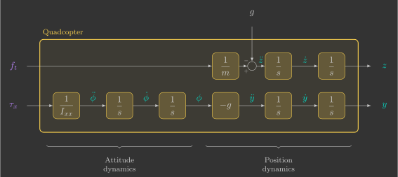
This becomes clear when the equations are represented as a block diagram:

Notice the following:

  • The thrust force \({\color{var(--c2)}f_t}\) is integrated twice to obtain the vertical position \({\color{var(--c1)}z}\) (Newton's second law for translation), acting independently on the vertical dynamics.
  • The torque \({\color{var(--c2)}\tau_x}\) is integrated twice to obtain the pitch angle \({\color{var(--c1)}\phi}\) (Newton's second law for rotation), and integrating twice more yields the horizontal position \({\color{var(--c1)}y}\).
  • Therefore, the transfer from \({\color{var(--c2)}\tau_x}\) to \({\color{var(--c1)}y}\) contains four integrators in series. This quadruple integrator results from the coupling between the rotational dynamics and the horizontal translational dynamics.
  • The negative sign in \(-g\) arises from the chosen axis convention: a positive rotation about the \({\color{var(--c1)}x}\) axis produces a negative acceleration along the \({\color{var(--c1)}y}\) axis.